Predicting Building Performance under Extreme Climate Conditions

Energy-saving building retrofits on the efficient frontier.

Thanks to everyone at Greiner, especially the other auditors, who cared enough to help advance the knowledge of building performance.

Environmental Economics

During my undergraduate education (2006-2009), I majored in environmental economics. More than once I was challenged with the following question: “Isn’t what’s good for one bad for the other?”

Well, it depends. There are trade-offs between personal consumption and public goods like clean air. However, what’s good for the economy can also be good for the environment.

Energy Efficiency

In Saving Energy, Growing Jobs, author and economist David Goldstein offers a set of policy proposals around energy efficiency, demonstrating that energy efficiency standards may offer a free lunch by incentivising emergent, innovative technologies and best practices which increase economic growth while reducing energy usage and related negative environmental externalities.

My interest in energy efficiency led to my first full-time job as an energy analyst in the residential construction sector. Over 20% of US energy use is in residential buildings. It turns out that energy efficient improvements to our homes are a vital part of our nation’s energy policy.

Designing on the Efficient Frontier

Within the residential energy sector, 62% of energy consumption is in heating, ventilation and air conditioning (HVAC). The way to minimize this portion of building energy usage is through energy-efficient engineering design.

West of the Rocky Mountains, here is a basic recipe for maximizing a building’s HVAC efficiency:

1. Reduce the building’s heating and cooling loads as much as possible through air sealing, insulation, dual-pane windows, etc.
2. Size the air conditioning system according to the building’s cooling load calculation whereby a smaller system would fail to maintain the desired indoor air temperature during a heat wave.
3. Blast as many cubic feet of air (CFM) across the evaporator coil as possible, which minimizes the energy wasted on dehumidification.

The chart below visualizes this process. At a 95 °F outdoor air temperature, a 3 ton air conditioner provides 26 kBTUh of sensible cooling capacity. By increasing the CFM, the sensible cooling capacity increases to over 31 kBTUh- a 15% boost in cooling efficiency.

This is Goldstein’s free lunch in action: the same equipment, designed to higher standards, yields improvements energy efficiency and comfort.

Market Failure

The process seems simple enough: a contractor performs a cooling load calculation (typically in energy modeling software) which tells them what size air conditioner to install in order to maximize equipment efficiency while maintaining the desired indoor air temperature.

Yet research shows that most HVAC systems in California are over-sized by 25% or more relative to their modeled cooling load calculation. Not only does this eliminate the efficiency boost, but it substantially degrades equipment durability and indoor air quality.

So why are HVAC systems typically oversized? There are many reasons, but the fundamental explanation is that contractors are afraid of installing equipment that may fail to keep a building cool during a heat wave.

It’s easy to understand this uncertainty. Cooling load calculations are meant to simulate a building’s cooling needs at outdoor air temperatures of over 100 °F. At these extreme temperatures, how much trust would you put in a computer simulation?

The purpose of this analysis is to show how buildings actually perform under extreme outdoor air temperatures in order to build confidence in the HVAC system sizing process, thereby improving building energy-efficiency and moving society to a more sustainable energy future.

Measured Performance

During the summers of 2016 and 2017, data loggers were installed on n = 22 different air conditioner condensers. The data loggers measured the condensers’ amperage draw every minute over an average study duration of 60 days. Each system went through at least one heat wave where outdoor air temperatures exceeded 100 °F.

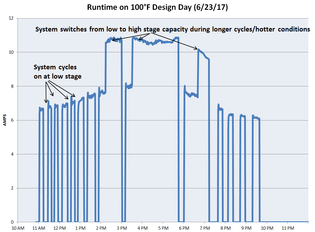
A visualization of a day’s worth of amperage measurements for a single two-stage system is provided below:

Based on the model and size of the condenser, the air conditioner’s cooling capacity is inferred using available engineering data.

Using this data, we can measure the building’s actual cooling load (as apposed to the modeled cooling load) because the heat energy removed by an air conditioner is equivalent to the cooling needs of the building.

Cyclical Cooling Loads

In order to compare each building’s actual cooling load to its model, I constructed a key performance indicator called the cyclical cooling load (CCL).

The crucial aspect of the CCL is that it aggregates data at the system cycle level. (In the previous plot, we can see that the system cycled on 14 times throughout the day.)

Here’s how it works: for each cycle, the minute-by-minute cooling capacity is aggregated. For example, a 36 kBTUh air conditioner that runs for 15 minutes would provide 8 kBTUh of cooling for that particular cycle.

The cyclical cooling capacity is then divided by the building’s modeled cooling load. This allows us to understand each building’s performance relative to its model while also standardizing the CCL across the disparate buildings in the study.

Continuing the example, a cycle that provides 8 kBTUh of cooling in a building with a 32 kBTUh cooling load will have a CCL of 0.25. The formula for the CCL is below: \begin{align} {x}_{jk} = {CCL}_{jk}= \frac{\sum_{i=1}^n y_{ijk}}{z_k} \newline \end{align}

y is the minute-by-minute measurement of the condenser’s capacity, which is aggregated over all measurements i for each system cycle j and system k, which is then divided by the modeled cooling load z of building k.

For each cycle, the cyclical cooling load has the following interpretation:

• CCL < 1 indicates that the building’s cooling needs are less than the modeled cooling load. This is typical for most cycles on most days.
• CCL = 1 indicates that the building’s cooling needs exactly match its modeled cooling load. Should the installed system capacity match the modeled cooling load, then the system (a “rightly-sized system”) will run for exactly one hour.
• CCL > 1 indicates that the building’s cooling load exceeds its modeled cooling load and that a rightly sized air conditioner will run for over an hour.

The research question of interest, re-framed in terms of the CCL, asks “What size CCL can we expect under extreme conditions?”

The Generalized Extreme Value Distribution

Over the duration of the study, each climate control system had over 1000 cycles on average, which means potentially over 1000 measurements of the CCL.

We can use the variation in CCL measurements to refine our question and ask, “What value CCL occurs 1% of the time or less?”

In order to answer this question, I fit a Generalized Extreme Value distribution (GEV) to the data. The history of the GEV distribution extends back to 1928 when Fisher and Tippet demonstrated that regardless of the underlying probability distribution of the random variable X, the probability distribution for the last order statistic converges to the GEV distribution.

There are several methods of fitting a GEV model to data. Given the nature of this data set, the tail behavior of the exceedances are modeled using the Generalized Pareto distribution.

\begin{align} f(X|\mu, k, \sigma) = \frac{1}{\sigma}(1 + k \frac{x-\mu}{\sigma})^{-(1/k + 1)} \newline \end{align}

The model finds the optimal values for the location parameter k and the scale parameter σ, while the threshold parameter μ is estimated from the data by studying the linearity of the exceedences.

Probability Model

The probability model is coded in Stan. As Stan does not contain built-in functions for the Generalized Pareto Distribution, the log-likelihood probability density (derived below) is included in the function block:

\begin{align} f(X|\mu, k, \sigma) = \frac{1}{\sigma}(1 + k \frac{x-\mu}{\sigma})^{-(1/k + 1)} \newline \end{align}

\begin{align} ln(f(X)) = -(\frac{1}{k}+1) ln(\frac{1}{\sigma}(1+k\frac{x-\mu}{\sigma})) \newline ln(f(X)) = -(\frac{1}{k}+1) * ln(\sigma^{-1})+{log1p}(k\frac{x-\mu}{\sigma}) \newline L=-(\frac{1}{k}+1) \sum_{i=1}^n log1p(\frac{k}{\sigma}(x-\mu)) -Nln(\sigma) \end{align}

Because there are multiple buildings to be modeled, the model block incorporates a ragged data structure and runs in a for-loop.

Individual Effects Model

There are several ways to characterize any probability distribution depending on the research question of interest. What we want to know is the probability of getting a CCL as extreme as X or greater. Given this framing of the research question, it makes sense to examine the complementary cumulative distribution function (CCDF), an inverse of the cumulative distribution function where higher values of X have decreasing probabilities.

The individual effects model fits a separate CCDF (the blue curve) for each of the 22 systems. The models clearly fit the data well, even at the 1% probability threshold.

Despite the accurate model fit for each building, there is still variation in the CCL across buildings. Many buildings have a 1% threshold CCL of 3 or 4, while others are equal 10 or greater!

This variation among buildings encompasses the variation in both energy modeling and in in-field performance including HVAC sizing and design, installation quality and homeowner operation.

Multilevel Model

What we really want to know is the performance of the average building across all possible buildings. In order to estimate these singular parameters, I fit a multi-level model to the data.

A Bayesian multi-level model assumes that each of the parameters for the individual buildings have their own shared Gaussian prior distributions. The parameters of these prior distributions, which are themselves random variables, represent the quantites of interest.

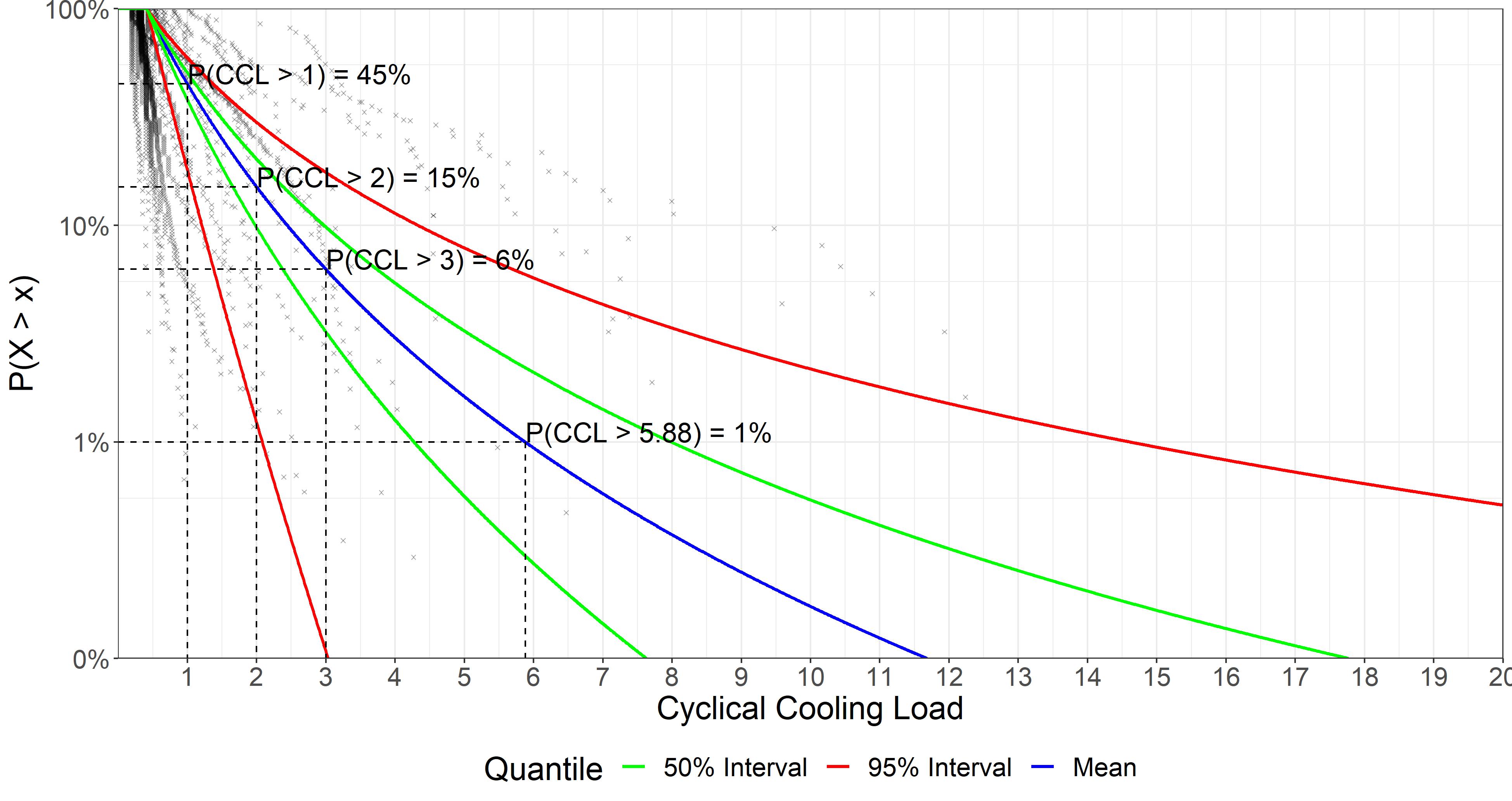
The CCDF for the multi-level model is below. The colored lines represent different quantiles on the parameters’ posterior distributions while the dark points are the data for all of the buildings in the study. (I recommend opening the image in a new window for a higher resolution view.)

We can see that the CCDF for the mean cuts roughly down the middle of the data although it is pulled to the right by the larger CCLs to the degree of frequency with which those values occur.

The key results from the study are as follows (with 50% probability intervals):

99% of the CCL’s are less than 5.88 (4.28, 7.98).

A rightly-sized system will run for 5.88 hours under the most extreme conditions.

The median CCL is 0.92 (0.82, 1.01).

During a heat wave, a rightly-sized system will run for about an hour at a time.

A CCL of 1 or greater occurs with 45% of the exceedances (0.38, 0.51)

During a heat wave, a rightly-sized system will run for an hour or more on 45% of the cycles.

With these expectations in mind, a contractor can confidently understand how their system will perform under extreme weather conditions when it is accurately sized for the building.

Follow-up Study

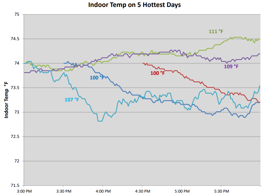
All of the customers in the study were highly satisfied with the performance of their HVAC system in terms of comfort and energy efficiency. Several customers with rightly-sized systems had their indoor air temperatures monitored to ensure that their home maintained a comfortable temperature during heat waves.

We can see that this system maintained 74-75 °F indoor temps (the specified design temperature) even on the hottest days of the year.

Works Cited

Coles, S (2001). “An Introduction to Statistical Modeling of Extreme Values.” Springer Series in Statistics. Springer Verlag London.

Ribatet, Mathieu. “The POT Package: An R Package to Model Peaks Over a Threshold.” http://pot.r-forge.r-project.org/

Vehtari, Aki. “Extreme value analysis and user defined probability functions in Stan.” https://mc-stan.org/users/documentation/case-studies/gpareto_functions.html

GitHub repo here.